Reverse engineering David Goodsell

Introduction

For some time I have been interested in the relationship between art and structural biology. In particular, I am fascinated by the various ways of representing three-dimensional structures of biological macromolecules, either by computer graphics, animations, or tangible, physical models.

Like many people, I like the unique style in which David Goodsell illustrates the structures of the Molecule of the Month (MotM) section in the Protein Data Bank. However, reproducing the way he renders molecules is not a straightforward task. To generate the figures in MoTM Goodsell uses some software he developed (apparently in Fortran, according to this German link). There are several tutorials and tools to emulate his rendering style¹, but none of these fully convince me. However, I took some ideas from them and managed to develop two methods using PyMOL. At first I just wanted to get an idea of how to do some figures with Goodsell’s style, but it became kind of an obsession. I hope you will find this post useful.

An easy way using just PyMOL

To begin with, I will reproduce the figure that appears on the September 2000 entry of MotM, corresponding to hen egg white lysozyme (PDB ID: 2LYZ).

First load the structure of 2LYZ (for example by using fetch 2lyz), then remove the water molecules with remove solvent , display the protein as CPK spheres with show spheres, put a white background with bg_color white and color the atoms by element according to the classical scheme (carbon in white, nitrogen, oxygen and sulfur in blue, red and yellow, respectively).²

color white
color lightblue, name N*
color blue, resn ARG+LYS and sidechain and name N*
color salmon, name O*
color red, resn GLU+ASP and sidechain and name O*
color sulfur, name S*

Once the scene is prepared, a simple way to get the figure is using the following commands:

unset specular
unset depth_cue
set ambient, 0.6
set ray_trace_mode, 1
set ray_trace_depth_factor, 1
set ray_trace_disco_factor, 1

After rendering with ray, something like this appears:

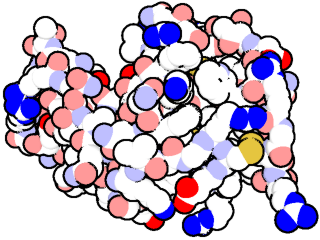
It may be necessary to adjust the ambient variable to get rid of the shading on the spheres.³ Besides, depending on the render size, ray_trace_gain has to be modified to alter the thickness of the borders.

A more complex method

Bonnie Scott published a while ago a tutorial where she uses two methods to achieve Goodsell’s style. One uses Chimera, while the other uses a combination of ePMV and Cinema4D. Both approaches consist in rendering colors, shadows and outlines separately, and then merging them using a graphics editor such as Photoshop. I will adapt this strategy to PyMOL. This method is more cumbersome than the previous one, but allows more control over the end result.

In this instance I’m creating the image of an antifreeze protein from the beetle Rhagium inquisitor (PDB ID: 4DT5). First load the structure and prepare the scene:

hide all
remove solvent
remove hetatm
show spheres, polymer
unset depth_cue
unset specular
unset ray_shadow
set ambient, 1
bg_color black

Then render:

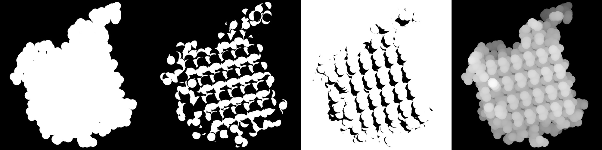
1. The alpha mask of the whole protein.

   color white, polymer
   ray 1000, 1000
   save protein.png
   

2. The alpha mask of nitrogen and oxygen atoms.

   color black, polymer
   color white, name N*+O*
   ray 1000, 1000
   save n+o.png
   

3. Shadows.

   bg_color white
   util.ray_shadows('black')
   set reflect, 1
   set reflect_power, 0
   color white, polymer
   ray 1000, 1000
   save shadows.png
   

4. And finally the z-buffer⁴.

   bg_color black
   set depth_cue
   unset ray_shadow
   set fog_start, 0
   clip atoms, 2, all
   color white, polymer
   ray 1000, 1000
   save z-buffer.png
   

With them the following images are obtained:

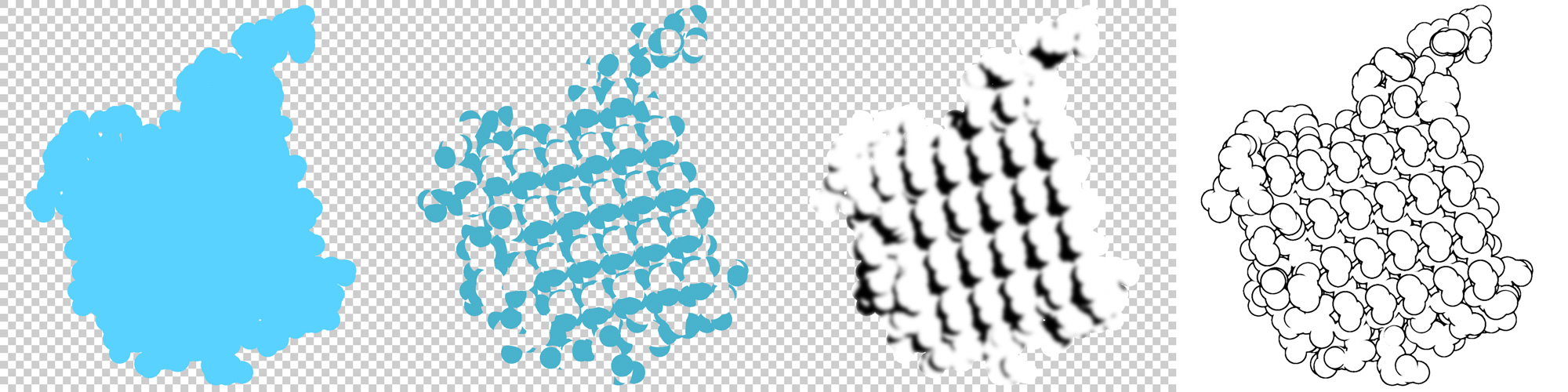
These have to be opened as layers in Photoshop, GIMP, etc. and processed as follows:

1. The alpha mask from the whole protein, the nitrogens and oxygens are transformed into a quick mask and filled with the chosen color.
2. This step is optional: Gaussian blur is applied on the shadows layer and then it is clipped to the alpha mask of the whole protein.
3. From the z-buffer the protein outline can be obtained using, for example, the Sobel operator in GIMP (Filters ‣ Edge-Detect ‣ Edge) or the Find Edges filter in Photoshop (Filter ‣ Stylize ‣ Find Edges). Then levels or curves need to be adjusted to remove the faint outlines from the inside of the spheres.

At the end of these steps, the layers should end up like this:

These are combined (borders and shadows are in Multiply mode) to get the final figure:

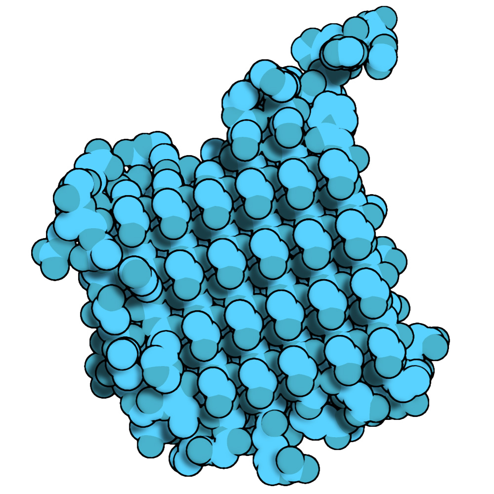
As you can see, this structure has a highly ordered array of threonines in charge of coordinating water molecules, stopping the growth of the ice crystals present in the cellular environment.

More information

If you want to know more about the work of David Goodsell, check out his web page, the section Molecule of the Month on the PDB or his book The Machinery of Life, which has many of his illustrations.